TL;DR (Abstract)

Here we summarize the article to provide a high-level overview. The modern ML field widely uses quantization to compress models and accelerate compute. How we actually quantize parameters centers around minimizing the quantization error. This error is not trivial to model, due to its dependence on the input signal. Our goal in this article is to explore a first-principles approach to derive the quantization error under a specific scheme (fixed point per-channel weight quantization). We model the input signal from its PDF, and use the observation that deep learning weights follow gaussian distributions, to simplify our model. Upon testing on Llama-7b's parameters, we find that a theoretical model using the gaussian assumption reasonably captures the quantization error distribution. Furthermore if the ratio of the quantization grid to distribution standard deviation ($q/\sigma$) is less than 2, we can accurately model the error as the addition of independent uniform noise.

Introduction

The basic procedure of quantization is pretty simple, but the ramifications of the process on a model's accuracy can be large and highly unpredictable. A good first pass we quantizers^[1] use to see how lossy a quantization scheme can be is to measure the error between full-precision and low-precision parameters. The intuition being if the error is large, then the post-quantized model will probably do badly on the task at hand. At my job, I would go through many, many, distribution plots of these errors to glean some patterns. As I merrily swiped through these plots, two questions would consistently come to mind:

1. Can we motivate the quantization error theoretically? In other words, can we model the error a priori without being handed a tensor of weights/activations first?
2. What exactly is the relationship between the error and actual model accuracy? We know there is one but how do we quantify it?

Beyond just my curiosity, these questions have practical implications too. If we can model the propagation of quantization error well enough without expensive runs of the model, we can attain a sense of where the model gets hurt the most, and work to contain them. If we can find the relationship between quantization error and model accuracy loss, we'll have much deeper insights into how the model learns, and will likely open new doors for how we can efficiently model data.

Unfortunately, question 2 is really challenging to answer, with various research groups approaching this from different directions^[2]. Thankfully, question 1 feels contained enough to tackle head on. To make life as simple as possible, let's focus first on fixed point (aka integer) quantization of a pre-trained model, where quantization bins are uniformly separated^[3].

The structure of this blog breaks down into two parts: theory and experiment. The theory is taken entirely from Widrow and Kollár's amazing classical exposition of quantization in their textbook (Widrow & Kollár). However, as this exposition is quite dense, I attempt to structure and summarize key ideas and equations, and having gone through most of the derivations myself, provide a little of my own commentary. I then design and run a series of experiments to verify the theory in the ML paradigm and identify extensions and limitations.

To narrow our problem scope even further , for now we just analyze the process of weight quantization. In general, weights play much nicer than activations (more stable, similar in distribution across layers), and make for a good playground to test our theory. The standard quantization procedure for model weights is symmetric quantization, which we describe briefly next.

Symmetric per-channel weight quantization

We can see how symmetric quantization translates full precision values to integer bins from Figure 1. This approach allows 0 to map to 0, so we no longer need a zero-point parameter.

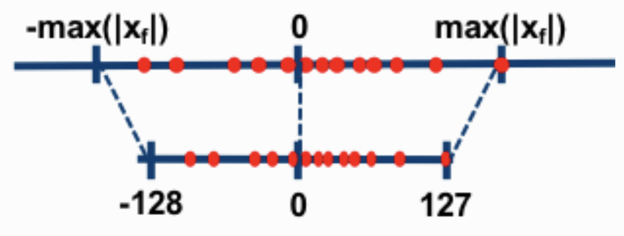
Figure 1. A visual of symmetric integer quantization. Image credit: Intel Labs.

The quantization grid size $q$ follows pretty intuitively. Given a channel $X_f$, our grid size $q$ is:

Given our grid size, we can calculate our quantized values as:

We're working with autoregressive language models, which primarily rely on the transformer architecture. As a result, the term 'per-channel' doesn't make too much sense, since we're no longer working with image channels. Instead we define each output neuron as a channel, which means each row of our weight matrix $W$ becomes a quantization 'group' (row since $W$ is typically defined as having dimensions (# output neurons, # input neurons)).

Modeling the Quantization Error

So given our quantization approach, what does the error induced by quantization look like? Notice from above that the lossy operation here comes from rounding. So we know that whatever quantized value $\hat{x}$ we have is within $\pm q/2$ of the original value $x$. But can we get more exact? It may be tempting to use the rounding information and model the quantization error as $\mathcal{U}(-q/2,q/2)$, where $\mathcal{U}$ is the uniform distribution. Many research papers take this approach (eg., (Meller et al, 2019), (Noune et al, 2022)).

However, a key detail about quantization is given the scheme and our input signal $x$, we can calculate exactly what our quantization error will be - it's not a stochastic process. This makes analyzing it really hard, as we don't have access to the input signals a priori (or if we do, it's sitting as a matrix of numbers, not an elegant mathematical formulation). As a result, the error can't blindly be modeled by adding some IID noise and calling it a day^[4].

Although the road ahead seems unclear, we can thankfully turn to the hard work done by electrical engineers over the last century to guide our understanding of quantization error. We'll find that there is still a lot we can learn from the rough approximation of uniform noise.

Before we go further, I found myself re-visiting similar topics while learning about this, so I'm writing out some key nuggets of knowledge about the Fourier Transform that we will refer to frequently.

Important Notes about Fourier Transforms (FT)

1. The Fourier transform represents a different (but entirely equivalent) view of a given function $f(x)$. It's easier to think about it in terms of time signals and frequencies, so let's say we have a time signal $x(t)$ (e.g., an audio recording) ^[5]. We can interpret the FT $\mathcal{X}\mathcal{(}\mathcal{w}\mathcal{)}$ , as the limit of a Fourier series - given our basis function as the standard sine wave, what combination and proportion of frequencies ($w$) do we need to add to get our original signal? The general expression for the transform is:

2. One of the most elegant results from Fourier theory is the Nyquist sampling theorem. Simply put, suppose the maximum frequency contained in $x(t)$ is $|F_{max}|$ Hz. You wish to sample the signal to compress it, so you sample it at a frequency of $W$ Hz. So long as $W\ge 2\ast |F_{max}|$ Hz, you can fully recover the original signal! In practice, this means you can tremendously compress the signal without loss, allowing for much faster computation and reduced memory footprint.
3. The probability distribution function (PDF) of a random variable $X$ has an equivalent representation $\mathrm{\Phi }(u)$, known as its characteristic function. The transformation $f_X(x)\to \mathrm{\Phi }(u)$ is just the Fourier transform of $f_X(x)$, and the transformation allows one to compute moments of $X$ much more easily. You can see an example of this as follows:

Similarly, for higher order moments,

Modeling the Quantization Process

Now, how can we represent the process of quantization? Let's look at sampling a signal (Figure 2). This idea is visually similar to quantization, but we want to bin values, not just sample them. Our problem is that the quantization process is deterministic given the input signal. This makes modeling the process theoretically to be quite tricky, as its entirely contingent on the signal. Following Woodrow and Kollàr, let's instead model the quantization process on the distribution from which the signal is drawn, treating a specific signal as a sample drawn from the distribution^[6].

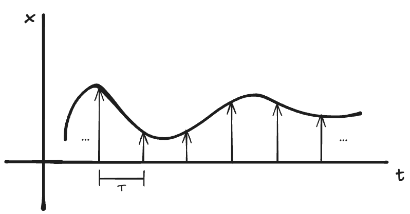
Figure 2. A signal being sampled at a frequency of 1/T Hz.

Suppose we start with the PDF $f_X(x)$ of a random variable $X$ as shown in Figure 2. Given our quantization grid (the ticks on the $x$ axis), any values within $q/2$ of a tick collapses to that value. Thus, we can model the PDF of our quantized variable $\hat{X}$ as a sequence of Dirac delta functions, with each one integrating to the area under $f_X$ for the corresponding quantization bin. Figure 3 visualizes the PDFs $f_X$ and $f_{\hat{X}}$.

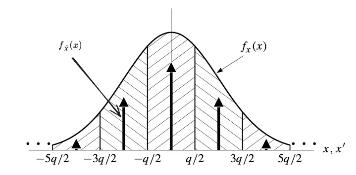
Figure 3. An example input signal distribution, and the corresponding distribution for the quantized output $\hat{x}$ modeled as a Dirac delta pulse train. Source: page 62 of (Widrow & Kollár).^e0a95a

Observing that this looks identical to sampling (with the modification that we're sampling areas rather than points on $f_X$), let's write out the expression for $f_{\hat{X}}$ as a pulse train of delta functions with the appropriate scales:

Now, squinting at this closely brings out the key insight. If we were to convolve $f_X$ with a uniform distribution and then sample it, we'll get the exact same resulting PDF. Let's define this uniform PDF $f_N$ as follows, visualized in Figure 4. Notice that $N$ represents the distribution for uniform noise.

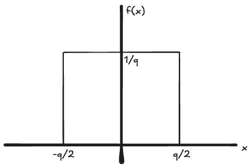
Figure 4. A graph of the uniform distribution, equivalent to a normalized window function.

Convolving $f_X$ with $f_N$ gives us the area under $f_X(x)$ within $[x-q/2,x+q/2]$ for all $x$.

Sampling this function at integer intervals of $q$ gives us the exact expression for $f_{\hat{X}}(x)$. So far, it seems as though we've just introduced a new random variable $N$, and manipulated our PDFs around to get the right answer. But recall that convolving two PDFs is simply adding two random variables together. We now see that we're actually adding uniform noise $N$ to our input signal $x$ to get $f_{X+N}(x)=f_X(x)\ast f_N(x)$, and then sampling this distribution to get our quantized PDF. Awesome! We finally have a formulation that takes a signal $f_{X+N}$ and samples it to get our output signal $f_{\hat{X}}$. Now we can take advantage of all the tricks that sampling theory has to offer, plus a few new ones. The intermediate PDF is known as the PQN model (pseudo-quantization noise) model for quantization. When the input distribution meets certain criteria (discussed below in #Two Key Properties of Quantization), statistical properties of $f_{X+N}$ translate directly to $f_{\hat{X}}$, and we can even model our deterministic quantization error as the addition of independent uniform noise.

Taking a step back, we now have an elegant formulation of the quantization process, and a method to find the PDF of a quantized signal $\hat{x}$. Our next goal will be to model the quantization error $ϵ=\hat{x}-x$. We can do this pretty easily by convolving $f_{\hat{X}}(x)$ with $f_X(-x)$, but we'll approach the challenge slightly differently to build some more intuition.

Two Key Properties of Quantization

Given our treatment of $f_{\hat{X}}(x)$ as a periodic sampling of $f_{X+N}(x)$ with "period" $q$, let's see what properties we can take advantage of. While there are several neat theorems that come out of this method, we highlight two primary ones that capture the main gist. Define $\mathrm{\Psi }=2\pi /q$, our radian sampling frequency. Then we can find the characteristic function of $\hat{X}$ from Eq (1) by taking its Fourier transform, resulting in:

The form of this equation is classic to sampling theory; the sampled function's Fourier transform (${\mathrm{\Phi }}_{\hat{X}}$) is an infinite series of shifted replicas of the input signals Fourier transform (${\mathrm{\Phi }}_{X+N}$). An example of this is shown below.

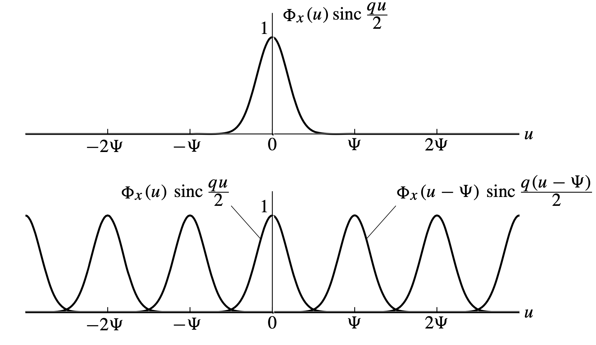
Figure 5. The characteristic function ${\mathrm{\Phi }}_{X+N}$ (top), and ${\mathrm{\Phi }}_{\hat{X}}$ (bottom), an infinite series of replicas of ${\mathrm{\Phi }}_{X+N}$ centered at integer multiples of $\mathrm{\Psi }$. Source: page 66 of (Widrow & Kollár).

Now, the following quantization theorems (QTs) follow intuitively:

1. QT I: If ${\mathrm{\Phi }}_x(u)=0$ for $|u|\ge \mathrm{\Psi }/2$, we can fully recover our input distribution given our quantized distribution. This theorem is identical to the Nyquist sampling theorem, and simply states that if our quantization grid $q$ is small enough, we can completely recover our input signal from the quantized signal. We can see this directly from Figure 5. If the replicas are spaced far apart enough, we can use a low-pass filter to snatch the replica at $l=0$, and recover our input PDF.
2. QT II: If ${\mathrm{\Phi }}_x(u)=0$ for $|u|\ge \mathrm{\Psi }$, we can fully recover moments of $X$ from moments of $\hat{X}$. From Figure, this is as if the replicas overlapped but not enough to affect the curvature of ${\mathrm{\Phi }}_{\hat{X}}$ at $u=0$, so the derivatives of ${\mathrm{\Phi }}_{\hat{X}}(u){|}_{u=0}$ match the moments of $X$. Furthermore, we'll soon see that if QT II holds, our quantization error follows the uniform noise model. Note that if QT I holds, QT II automatically holds.

Theoretical Quantization Error

To start off modeling $ϵ$, let's go back to Figure 2, and pick an example quantization bin at $1\ast q$. We see that all values within $q/2$ of the bin get clumped into it, so the distribution of error is determined by how far any input within the $+/-q/2$ window lies relative to the bins. Given our input distribution $f_X$, we can formulate an expression for the error distribution as follows:

Here, $m$ represents the bin number. So for a given $m$, the error distribution around the bin value is just the input distribution around that value within a $q/2$ window. We can take the distributions for all bins/windows and stack them together to get our error distribution. An alternative representation is given in line 2, the product of the window function and the sum across bins.

Next we compute our characteristic function for the error. This follows (Widrow & Kollár) chapter 5.1 for the mathematical derivation. At a high level, the product in the input domain leads to a convolution in the frequency domain between ${\mathrm{\Phi }}_N(u)$ (represented by the $sinc$ function) and a pulse train sampling of ${\mathrm{\Phi }}_X(u)$.

Taking the inverse Fourier transform of the characteristic function gives us a more powerful representation for the error distribution:

In both cases, notice the dependence on ${\mathrm{\Phi }}_X$ only at specific intervals - particularly, integer multiples of the quantization frequency (recall $\mathrm{\Psi }=2\pi /q$).

When QT I or QT II is satisfied, we see that all the non-zero integer multiples of ${\mathrm{\Phi }}_X(l\mathrm{\Psi })=0$, so we're left with just the term at $l=0$, implying the error perfectly follows the uniform distribution.

A key input distribution that we want to look at is the Gaussian. It's been observed and hypothesized many times that the pre-trained weight matrices fit to this distribution closely in LLMs, so it'll be useful to explore its properties under quantization further (Dettmers et al, 2023). Let's take a look at the characteristic function for a Gaussian, given its PDF:

Taking a quick look at this, we realize it doesn't fit any of the QTs as ${\mathrm{\Phi }}_x$ isn't band-limited! Nonetheless, we can go through the algebra to find a general form of the error distribution from Equation (1).

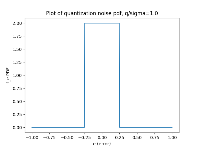
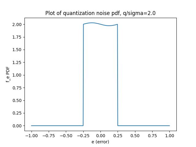
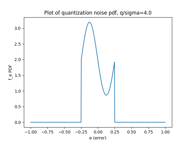
We can use the Jacobian elliptic theta function to numerically calculate this PDF for different values of $ϵ$. We can also find its first and second moments, taking initial terms in the infinite series as approximations (refer to section 11.9 for the full infinite series expansion[^6])

As the equations show, the key value to pay close attention to is the ratio of $q/\sigma$. For quantization grid sizes smaller than the input distribution's standard deviation, the exponent decays rapidly, and our error distribution mimics the PQN uniform noise model. As Widrow and Kollár observe, even for quantization grids up-to double the distribution's standard deviation ($q\approx 2\sigma$), the PQN model still reasonably applies. Let's see if we can replicate this observation. As a visual example, we plot the PDF for three cases: $q=\sigma$, $q=2\sigma$ and $q=4\sigma$. For $q=2\sigma$, the PDF deviates slightly from uniform, but not enough to change underlying behavior.

(a)	(b)	(c)

Figure 5. Plots of theoretical quantization noise with increasing grid sizes (decreasing granularity). The distribution moves away from uniform once $\sigma <q$. In all cases, $\mu =q/4$, inducing a phase shift in the oscillatory behavior of the distribution.

An interesting point to note is the sinusoidal behavior in the error distribution. It's only noticeable for large grid sizes, and mathematically, this stems from the $e^{j\mathrm{\Psi }ϵ}$ term in (2), which in turn stems from the shifted $sinc$ terms in ${\mathrm{\Phi }}_{ϵ}$. However, I have yet to find a good intuition for where this oscillatory behavior stems from.

As a first-pass and sanity check of our model, we sample gaussian data and compute the quantization error statistics, comparing it to the theoretical results. Below is a table summarizing the results. With a large sample size ($n=1e6$), the error statistics are closely matched by theory.

Experiments on Llama-7b

We've built up a good understanding of the theory, but how well does this actually apply to deep neural networks? Typically, real-world signals rarely follow a clean distribution that we can just plug-and-play with, but we're partially saved by the following observation: most neural network weights are normally distributed. If this is true, we can use our theory to directly model the quantization error, at least due to weight quantization.

Now, to be honest, beyond seeing this observation cited in papers every now and then, I haven't been able to find good verification as to why this hypothesis exists. Weights are generally initialized from a normal distribution, but I've always assumed the distributional shift over training would change their structure significantly. While I'm still digging for a good explanation of this, we can take inspiration from (Dettmers et al, 2023) and simply run significance tests on all our weight tensors to validate the claim.

Now let's look at Llama-7b. We select Llama-7b as it's an open-sourced and well-studied model, and is large enough to be respectable in today's world, but not so large that experiments become expensive to run. As Dettmers shows, a lot of interesting results occur at the 6.7B+ parameter range, so we don't want to pick too small of a model. We follow their approach to look at per-channel weights, and find that they're reasonably gaussian. Running the Shapiro-Wilk test with a 5% significance level tells us that 85% of weight channels are approximately gaussian^[7] (Dudley, 2012). This is slightly different from Dettmers' reported result of 92.5%, although differences in model versions used could account for this. We note that all the Layernorm weights fail this test, and plotting some of their histograms indicate a far-from Gaussian shape - all of them have extreme outliers, as demonstrated by the large kurtosis (see Figure 6). Unlike linear layers, Layernorm weights are initialized all to ones, so this likely affects the distribution over training to be further from gaussian. This initialization also means the center of the distribution is no longer 0, so our symmetric quantization scheme would end up wasting a lot of bins that are empty.

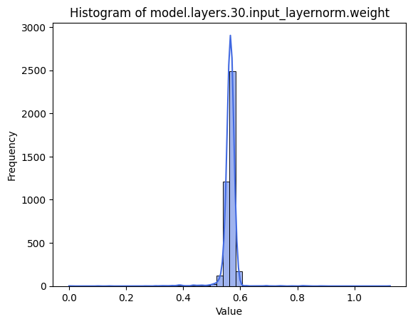
Figure 6. A histogram of a selected Layernorm. The distribution's skewness is -2.5, and excess kurtosis of 103.2.

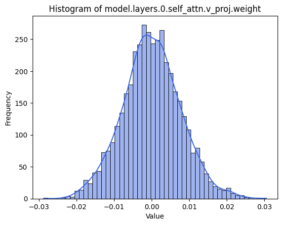
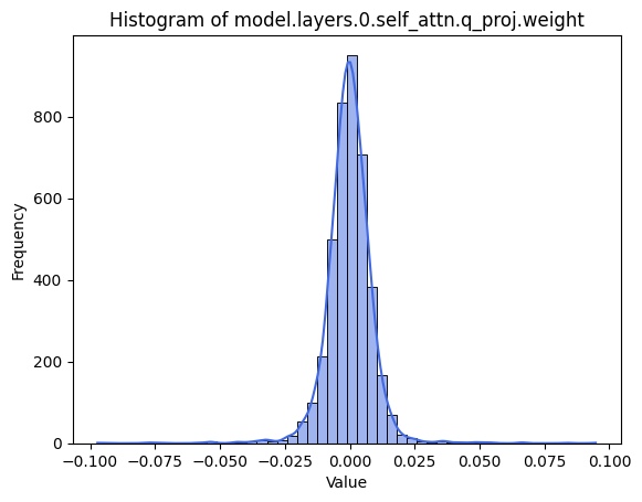
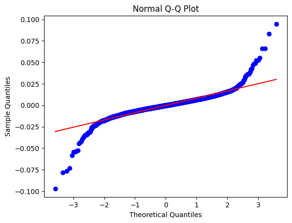
Among the remaining parameters, we note that they all have a symmetric, bell-shaped curve (see Figure 7). Let's take a look at an example failure mode of weights that don't fit the gaussian. The outliers aren't as extreme as in the case of the Layernorm - we can visualize the outliers-induced heavy tails via the q-q plot of the data relative to a theoretical gaussian distribution. The story of the outlier is incredibly interesting in the quantization space, and one that I'll dive into in my next post. For now, however, we posit that these outliers are minor enough to continue using the gaussian model, and proceed with our attempt to predict quantization error using our model.

(a)	(b)	(c)

Figure 7. In (a) A histogram of a selected Attention weight matrix that fits to a gaussian. The distribution's skewness is 0.1, and excess kurtosis of 0.2. In (b), an example weight distribution that doesn't fit to a gaussian distribution, and its corresponding q-q plot (c). The tails are heavier than expected due to outliers, but not as extreme as Layernorm weight distributions. Here, the skewness is still small at -0.2, but the kurtosis is larger, at 16.7.

For each weight channel, we compute the mean and standard deviation as follows, and set the theoretical distribution to be $f_X(x)\sim \mathcal{N}(\overline{X},{\overline{\sigma }}^2)$. We then use equations (3) and (4) to find our theoretical error moments. Next we compute our actual errors by quantizing the weights to $n$-bit fixed point precision, and compare the resulting statistics for various $n$.

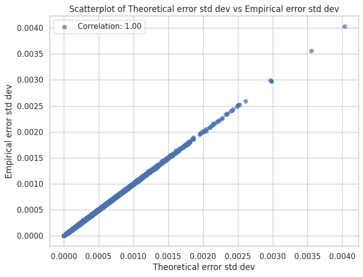
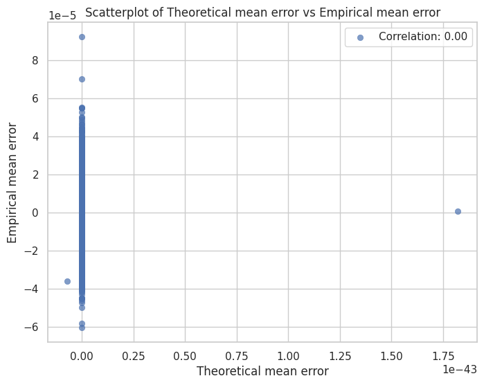
We compute the error moments for all the non-Layernorm layers, and plot these in Figure 8a and 8b, which show scatterplots with theoretical standard deviation and mean error vs empirical results. We find that our model explains the variance of quantization error quite well!

(a)	(b)	(c)

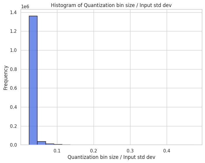
Figure 8. Plots of theoretical predictions of the quantization noise statistics against empirical results. Here, $\text{nbits}=8$. (a) and (b) show the correlation in standard deviation and mean of theoretical and experimental error. (c) shows a histogram of $q/\sigma$ ratios for all the weight channels.

We also try testing the empirical standard deviation against that predicted by purely uniform noise and continue to observe a perfect correlation. Given the small $q/\sigma$ ratio, this makes sense as the auxiliary exponent terms in eq (2) drop off very quickly, allowing for a near-uniform approximation to our noise.

However, the prediction of the mean of the error is much poorer and spread out, likely due to the asymmetry of the actual values that the gaussian model doesn't account for. Nevertheless, the error is quite small (~1e-5). We also observe that most of the channels have small quantization grid sizes relative to the input variance, as seen in Figure 8c.

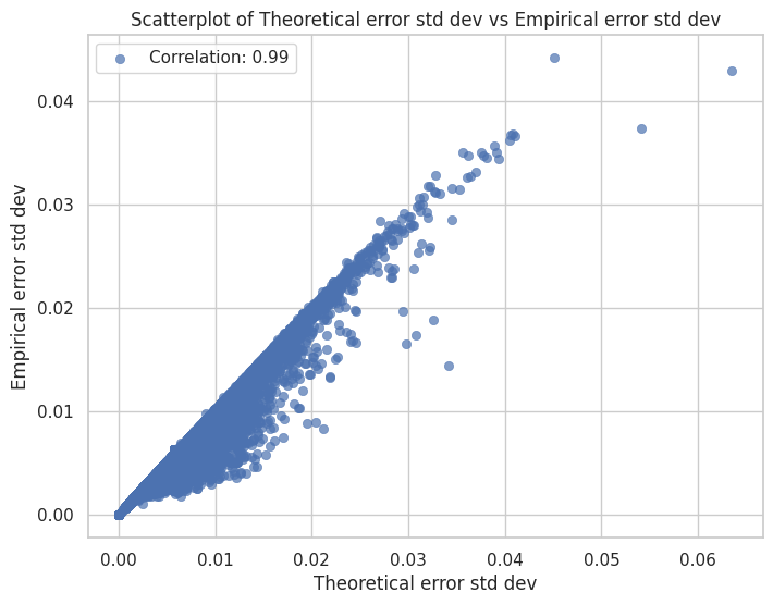
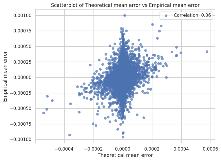
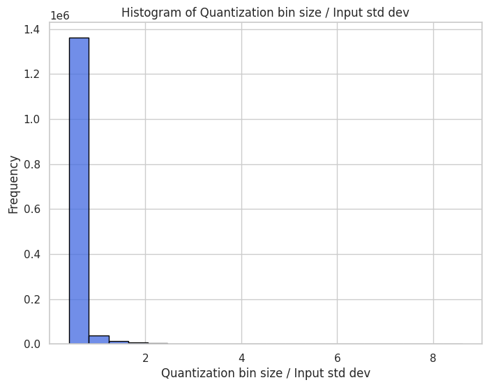
Next, let's take a look at the 4-bit quantization case. Seeing Figure 9, we observe that the theoretical error variance prediction predicts the empirical values well, but consistently underestimates them. This is a really interesting find that we'll come back to. In the meantime, we also see that the mean of error predictions are just as bad as in the 8-bit case, if not worse. The positive correlation is vaguely present, and most of the mean errors do fall close to 0. The worst gap in prediction is on the order of 1e-3, which is still relatively small but worryingly larger than in the 8-bit case, where the biggest gap was 8e-5.

Finally, we note from Figure 9c that the quantization grid sizes are larger relative to the input variance than in the 8-bit quantization case. In a few cases the bin size can be as large as three times the standard deviation.

(a)	(b)	(c)

Figure 9. Plots of theoretical predictions of the quantization noise statistics against empirical results. Here, $\text{nbits}=4$. (a) and (b) show the correlation in standard deviation and mean of theoretical and experimental error. (c) shows a histogram of $q/\sigma$ ratios for all the weight channels.

Now, let's come back to the interesting underestimate in Figure 9a. Initially we thought our approximations for and were too steep, so we tried adding some more terms from the infinite series (see section 11.9 in (Widrow and Kollár et al)). However, this didn't change the results at all. Investigating more closely, we hypothesize the underestimation is likely due to distributional differences between the actual data and the normal curve. As we've seen, the weights generally have heavier tails (due to more outliers) than the gaussian distribution would predict. With fewer output bits, the bin/grid size gets bigger, so a lot of the outliers get dumped into the same bins as the 'in-distribution' values, causing the empirical error to increase. Since our model distribution doesn't have these tails, we underestimate the error.

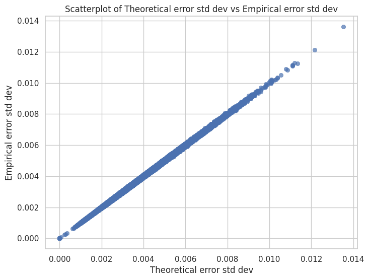
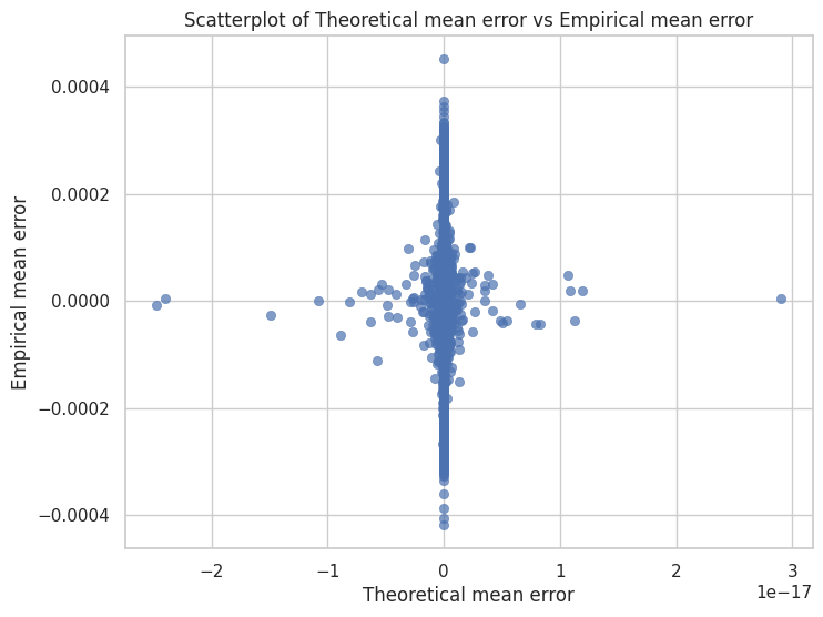
To test this theory, we try re-running the predictions excluding the heaviest tail channels. This eliminates the ~15% of the weight channels that failed the normality test. Our results in Figure 10a show a far improved correlation, reinforcing our theory. Interestingly, we see a return to a bias towards predicting 0 as the theoretical error mean, shown in Figure 10b.

(a)	(b)

Figure 10. Removing the channels that failed the normality test, we find that the correlation between theory and experiment is much closer in the $\text{nbits}=4$ case. (a) shows the standard deviation correlation, while (b) shows mean correlation.

So, what have we learnt from this analysis? First, we find that although the data structures don't satisfy all the assumptions we made in theory (IID gaussian), our general noise model does a pretty good job predicting the variance in empirical quantization error. We also found that it's much more sensitive to predicting the mean error, however, showing the gaps between our assumptions and reality.

Now, although the fit between theory and experiment is promising, one look at equation (2) gives me the shivers. Once we bring in a formulation for activation quantized error, modeling the error propagation through a network is going to be gnarly. What we really want to know is if we can use the PQN model to substitute the error with uniform noise. Based on the last part of our theory section, we know this all hinges on the critical $q/\sigma$ ratio. From the last section we saw that if $q/\sigma >2$, the PQN model starts to break down. Figures 8c and 9c show that most channels have ratio under 2. Let's look at this more closely.

A couple of key hidden details in our experiments

A critical difference between quantizing real model weights and working in theory is our quantization bins are no longer infinite. Depending on the scheme we use, we could encounter clipping, which introduces an entirely new form of error. However, since we're using min-max quantization, we don't have to worry about not finding a nearest bin for any value. Thus, we treat the weight tensor as if it has an infinite quantization grid. Nonetheless, we can expect discrepancies between our results due to this difference.

Also, since we're using symmetric quantization, our quantization grid is centered at 0. If it wasn't we would need to add a phase shift to our results^[8]

On the Applicability of the PQN Model

Given the data is normally distributed, when does our uniform noise approximation break down? Let's explore the key ratio $q/\sigma$ a bit further. We can easily find our quantization grid size as they are just the quantize scales using the symmetric quantization paradigm. Let $C=2^{n-1}-1$. We then see that:

From the previous section, given an inputs are $\sim \mathcal{N}(0,{\sigma }^2)$, we know the uniform noise model starts to collapse when $q>\sigma$. We can imagine this could happen when there are a few large outliers, but not enough to skew the input distribution's variance. We can find our weight's variance as follows, where we utilize the symmetry of the gaussian to center it at 0. Experiments show that this holds for most weight channels, where the largest channel mean value for Llama-7b was 0.003, small enough to validate our approximation.

So when will $q>2\sigma$? Squaring both sides and substituting their definitions, we find that

It's easy to see that when $4C^2>N$, this inequality is impossible to attain. Essentially, when the size of the weight matrix being quantized is small, we'll always be able to approximate the quantization error with uniform noise. Supposing $N$ is large enough, we obtain the following requirement for the collapse of the PQN model:

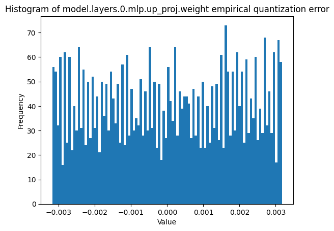
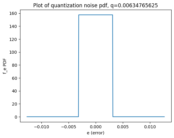
For attention projection matrices in LLaMA under 8-bit per-tensor quantization, $\frac{N}{C^2}-1\approx 1000$^[9]. In this case, so long as we have a large outlier in our midst, the PQN model will start to break down. However, if we use per-channel quantization, $N$ becomes much smaller, rendering the inequality impossible.

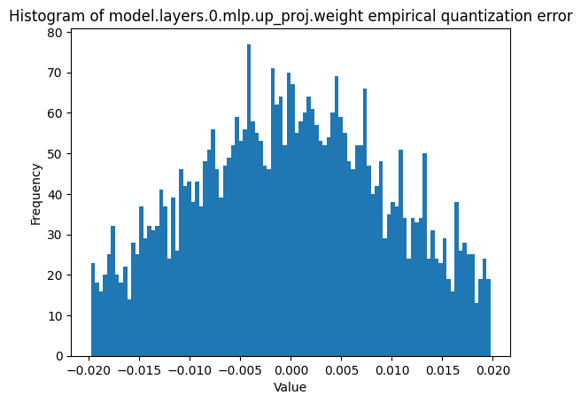
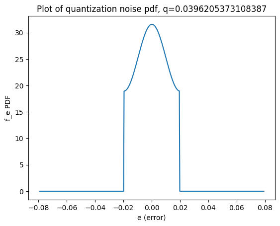
Alternatively, if we're quantizing to smaller bit sizes, $C$ exponentially shrinks, making the inequality easier to satisfy. We can see this from the histograms of Figure 11 and 12, where in the 4-bit case there are a decent number of channels that exceed the $q/\sigma$ ratio to well past $2$. In contrast, the 8-bit per-channel quantization guarantees that $4C^2>N$, so we can safely use the uniform noise model. We show the histograms of two extreme channels and their corresponding theoretical PDFs. Along with noting a good match between the predicted and actual distributions, we see that in the $q/\sigma =3$ case the distribution is far from uniform. In this case, the full theoretical model is required to capture the error distribution. In the 4-bit quantization, we observe ratios as high as 8.6.

(a)	(b)

Figure 11. A side-by-side of theoretical and empirical error distributions for a particular weight channel, under 8-bit quantization. This is with $q/\sigma =0.4$.

(a)	(b)

Figure 12. A side-by-side of theoretical and empirical error distributions for a weight channel, under 4-bit quantization. This is with $q/\sigma =3.1$.

From these discussions and Figures 8c and 9c, we can take away the following: the uniform noise model (PQN) is surprisingly robust, especially in the case of per-channel weight quantization. The breakdown of the model in the per-channel case depends entirely on the presence of outliers that can skew the distribution tails. These seem to occur rarely (in the 4-bit case, only about 0.53% of weight channels have $q/\sigma >2$. In the 8-bit case, none of the channels exceed the inequality).

Conclusions

To wrap up, let's list our overall findings:

Theory:

• The quantization error model is built on modeling the input distribution of values. From this we can formulate a process that gives us the distribution of quantized outputs and errors, letting us calculate error statistics for actual data.
• Under certain assumptions, we can mimic the process as if we were adding uniform noise to our data. This is known as the PQN model (pseudo-quantum noise)
• Although the gaussian distribution doesn't satisfy the key assumptions of this PQN model, when the quantization grid is small enough, we can effectively still use the PQN model.

In our experiments, there are two axes that we're using to see if theory works well in practice. The first is to see if the gaussian approximation to weights give reasonable statistics. The second is to see if the stronger assumptions for the PQN model give reasonable statistics in practice.

Experiment:

• The Gaussian approximation to weights let us use our theoretical model works well to model second-order statistics for our quantization error, and gives a rough approximation to first-order statistics as well.
• We find that when there aren't too many outliers, the PQN model works great to model the noise. This can simplify the overall analysis tremendously since we can just use uniform noise additions rather than propagating our error distribution through the network.

Now, how can we expand this? An immediate thought is to test it on activations. Unfortunately, unlike weights, activations don't follow a particular distribution, significantly complicating our analysis. However, we might still be able to use the ideas here to capture activation error propagation through the model. We could try looking at how the weight errors cascade through the network to deviate activation values.

Another area to explore is when catastrophic model degradation occurs - does it happen through a series of accumulated smaller quantization errors, or a few large errors with outliers? If it's the latter, modeling the distribution becomes much harder since we need to capture the presence of such outliers.

I hope to follow up with this soon!

Thanks for reading to this point! I'm always looking for feedback, and would love to hear some if you have any. Stay tuned for future posts!

Footnotes